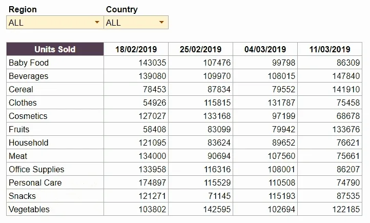
How to make a dynamic dashboard using Google Sheets

Cascading Menus: The second drop-down (Country) updates based on the selection of the first drop-down (Region)

Imagine you are a start to mid-level analyst or manager at a highly data driven organization. Part of your routine work is to deal with the same set of data, churn actionable insights from it and report it to a broader team. If expensive BI tools like Tableau and Qlikview are overkill for your requirement, then read further.

With the power of Google Sheets, anyone can create functional and dynamic dashboards which can be shared with a number of people for consumption. In this tutorial, we will make a simple dashboard using google sheets.

Note: You can create a similar dash in MS Excel as well with slight modifications,
but we will cover the various excel equivalents for Google Sheets functions in a later tutorial. You can also use the powerful Pivot Tables to create similar summaries, however, those are limited in functionality and not ideal to share with others in form of an intuitive dashboard interface.

In this tutorial, we will learn the following:

Use a sample sales data to create a summary of “units sold” aggregated by “item type” and by week/month/year of the “order date”.
Create cascading drop-down menu filters. In a cascading drop-down, the the drop-down options of one drop-down change based on the selection in another drop-down.
Add an “ALL” option in the drop-down filters to select multiple values. Use conditional formatting to highlight any input errors.
Share the dashboard with others in a “safe” way by protecting sheets
Next steps on how to make the dashboard more dynamic

Resources

Sample data

Courtsey E for Excel. Note that I updated the Order Date column to more recent dates.

Final Dashboard

In Google Sheets

List of major functions we will learn about:

Getting Started

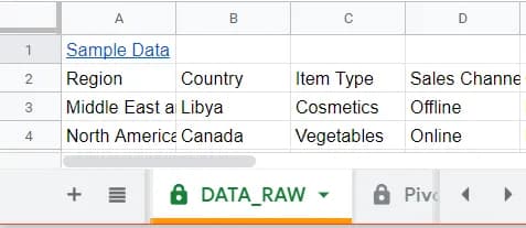
Copy and paste the sample data into a back-end sheet. As a good practice, I prefix my back-end data sheets with “DATA_” and also give them a unique sheet color.
Also create a new tab and call it “Summary” where all the action will happen.

Define Values, Dimensions and Filters

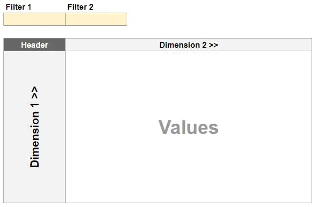
For the rest of the tutorial, we will use the following terms:

Values: The values/metrics which you want to see aggregated. Eg. Number of Units Sold, Total Revenues , Profit per Unit etc.
Dimensions: The dimensions across which the values will be aggregated. In this example, I am aggregating # Units Sold across two dimensions: Item Type and Week in which order was placed (Monday of the week of order date)
Filters: Additional filters to slice the data. In this example, I am using Region and Country as two filters. Note that country is a complete sub-set of Region (eg. India will always fall under Asia region and never under any other region)

Pro Tip: I prefer to use a consistent color scheme for all input cells.
In this case the only “inputs” by a user are the values of the drop-down filters (Region and Country). Hence they are color coded in mild yellow to let the user know that it can be changed.

Once we have created a basic structure for your dash, we move to the fun stuff, creating cascading menu drop-downs for your filters.

Creating cascading drop-down menus

First we create the list of items for the first drop-down (Region). The way data-validation based drop-downs work in Google Sheets is that they display a unique set of values from a selected range, in the same order as the values appear in the range. In our sample dashboard, we prepare the Region list by first getting a unique set of values of the Region column from our RAW_DATA sheet, and then sorting the output in alphabetical order using the sort function. We populate the sorted results in Cell A6 of the Summary sheet.
Notice that we have left a static value “ALL” in cell A5. I will come to that later.

=SORT(UNIQUE(DATA\_RAW!$A$3:$A$2002),1,TRUE) // first takes unique values from range DATA_RAW!$A$3:$A$2002 and then sort the results in alphabetical order

Puzzled by the varied use of the $ dollar sign in the formulas?
Read more about cell referencing in Google Sheets here

The last step is to populate these results in our Region drop-down on cell D3. For this, we select the cell D3, go to Data > Data Validation, under Criteria, select List from a range, and select the the entire range of values in Column A (‘Summary’!A5:A100). Make sure the “Show drop-down list in cell” option is checked. Once done, the list will start appearing in in cell D3 as a drop-down. Notice that blanks are ignored in the drop-down list and it shows up in same order (Alphabetical). 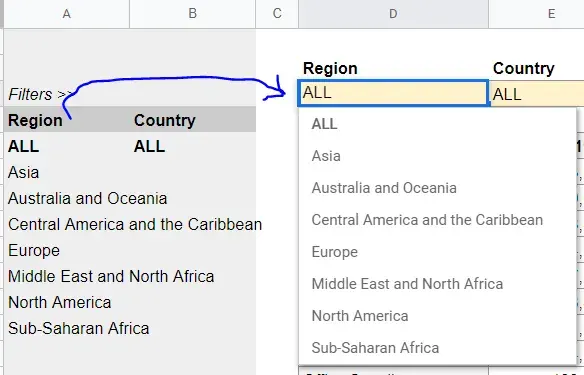Now, we use a similar formula to populate the values of our second drop-down (Country) in cell B6 of the summary sheet, but with one major difference: The values for Country drop-down should change based on what is selected in the Region drop-down. For this, we make use of the FILTER function. The sequence is as follows: First we filter for Country column values in RAW_DATA sheet conditional on the values in the Region column on the same sheet. Once we have the filtered Country values based on our selected Region, we apply the functions similar to our previous step to make our results unique and then sort them alphabetically Finally, for completeness I wrap our output inside an IFERROR function to ensure the Country list does not throw a Filter error when “ALL” is selected under Region. In case of such an error, I make the Country list empty. I also add a “ALL” static value in cell B5 (will come to its use later)

=IFERROR(SORT(UNIQUE(FILTER(DATA_RAW!$B$3:$B$2002,DATA_RAW!$A$3:$A$2002=$D$3)),1,TRUE),"")

// Select Country input values (DATA_RAW!$B$3:$B$2002) ONLY if the corresponding Region input values (DATA_RAW!$A$3:$A$2002) are equal to our currently selected Region in Summary ($D$3)

Now we again follow the steps similar to the Region drop-down, and use data validation to populate the Country drop-down in cell E3. Viola! we have the cascading drop-downs working, with the Country drop-down values changing based on the Region drop-down values.

Dynamically populating the dimensions (row and column headers)

Our original selection for row headers was Item Type and for Column headers was the Week containing the Order Date (A week is represented by the date on Monday of that week). Although for simple summaries where the dimension values don’t change, we can just manually populate static values for the two dimensions. However, for this exercise, I want both the dimension values to be dynamically populated from RAW_DATA For row headers, we use the same UNIQUE and SORT functions (refer to the previous cascading menu step) to populate all unique values of Item Type from RAW_DATA and also sort them alphabetically. For column headers, I want to populate the latest 4 weeks of data based on the Order Date in RAW_DATA.

In cell H5
=MAX(DATA\_RAW!$F$3:$F$2002) - WEEKDAY(MAX(DATA\_RAW!$F$3:$F$2002),3)

// MAX function pulls the largest date value (most recent) from
the range DATA_RAW!$F$3:$F$2002. Then we use the WEEKDAY function to subtract the number of weekdays past since Monday of that week. This way we always end up with the Monday of the week of Order Date, regardless of the date

Aggregating data based on your filters and dimensions

Finally, we use the versatile SUMIFS formula to conditionally sum the Units Sold column from RAW_DATA sheet. The conditions are applied on Region, Country, Item Type and Order Date SUMIFS in its simplest form is very simple to understand. Taking our example, we enter the following formula on cell E6 in Summary:

In Cell E6
=SUMIFS(DATA_RAW!$I:$I,DATA_RAW!$A:$A,_$D$3,DATA_RAW!$B:$B,_$E$3,DATA_RAW!$C:$C,$D6,DATA_RAW!$F:$F,">="&E$5,DATA_RAW!$F:$F,"<="&E$5+6)

The above formula explained in English is as follows: SUM the values in range DATA_RAW!$I:$I ONLY for selected rows where

Region is our selected region (DATA_RAW!$A:$A = $D$3)
AND Country is our selected country (DATA_RAW!$B:$B = $E$3)
AND Item Type is same as my current row’s header_Item Type_ (DATA_RAW!$C:$C = $D6)
AND Order Date is between Monday as per my current column’s header and Monday+6 (DATA_RAW!$F:$F,”>=“&E$5 & DATA_RAW!$F:$F,”<=“&E$5+6) Now we can drag this formula across our summary table. Just hide the Filter value columns A and B and that’s it! We have a functional dashboard!

Final touches to make the interface more user friendly

Using “ALL” option to select all Regions and/or countries:

In the SUMIFS function, if we use the asterisk (*) as a criteria value, the SUMIFS function ignores the entire criteria. So we need to tell the function to replace “ALL” value from drop-down with ”*” every time “ALL” is selected. The modified function is:

In cell E6
=SUMIFS(DATA_RAW!$I:$I,DATA_RAW!$A:$A,IF($D$3="ALL","\*_",$D$3),DATA_RAW!$B:$B,IF($E$3="ALL","\*_",$E$3),DATA_RAW!$C:$C,$D6,DATA_RAW!$F:$F,">="&E$5,DATA_RAW!$F:$F,"<="&E$5+6)

Add additional conditional formatting to highlight errors in drop-down values. In our example, if the user enters a value which is not part of the drow-down list, the color of the drop-down will turn from mild yellow to red to highlight the error.

For this, select the drop-downs at cell D3 and E3, go to Format > Conditional Formatting. Add something like this:
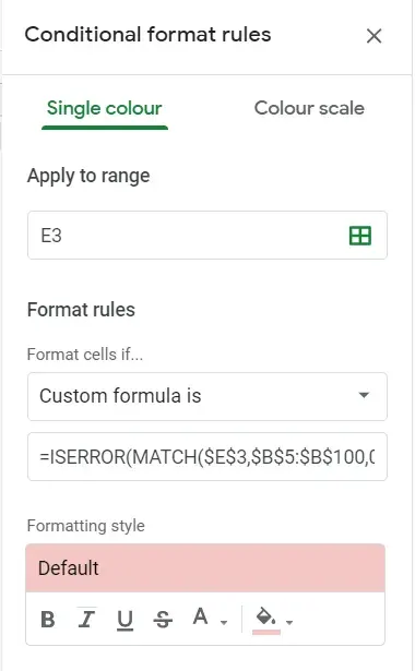
=ISERROR(MATCH($E$3,$B$5:$B$100,0))

Before sharing your new dashboard with others for consumption, you should protect the sheets so that other users cannot modify any formulas in the sheet. While you are protecting your sheet, add the Filter drop-down cells (D3 and E3) under exceptions (Except certain cells). This way, the only cells the users can change in the sheet are the ones that you want them to change. You can add more summaries of different values and dimensions. Some ideas based on the data in current example are:

Value = SUM of Profit / SUM of Unit Sold (profit per unit), Dimensions = by Week and by Country and Filter being Item Type in the drop-down
Measuring Average Lag between Shipping Date and Order Date: Value = Average of (Shipping Date minus Order Date), Dimension = by Order Priority and by_Item Type,_ Filters = Region and Country. In this scenario where were are aggregating as Averages, you should use AVERAGEIFS instead of SUMIFS

I hope this tutorial was useful and easy to understand. For any questions or feedback, you can comment on this post below.

~ Fin ~